This is an excerpt from an eBook on Sensor Fusion and Tracking that I wrote for Mathworks. They have graciously let me reproduce a portion of it for this blog. It has been modified and updated to improve clarity and to allow it to stand on its own apart from the rest of the eBook. You can download the full eBook here:
https://www.mathworks.com/campaigns/offers/understand-multi-object-tracking.html
This is a long post. Here is the tl;dr for those in a hurry!
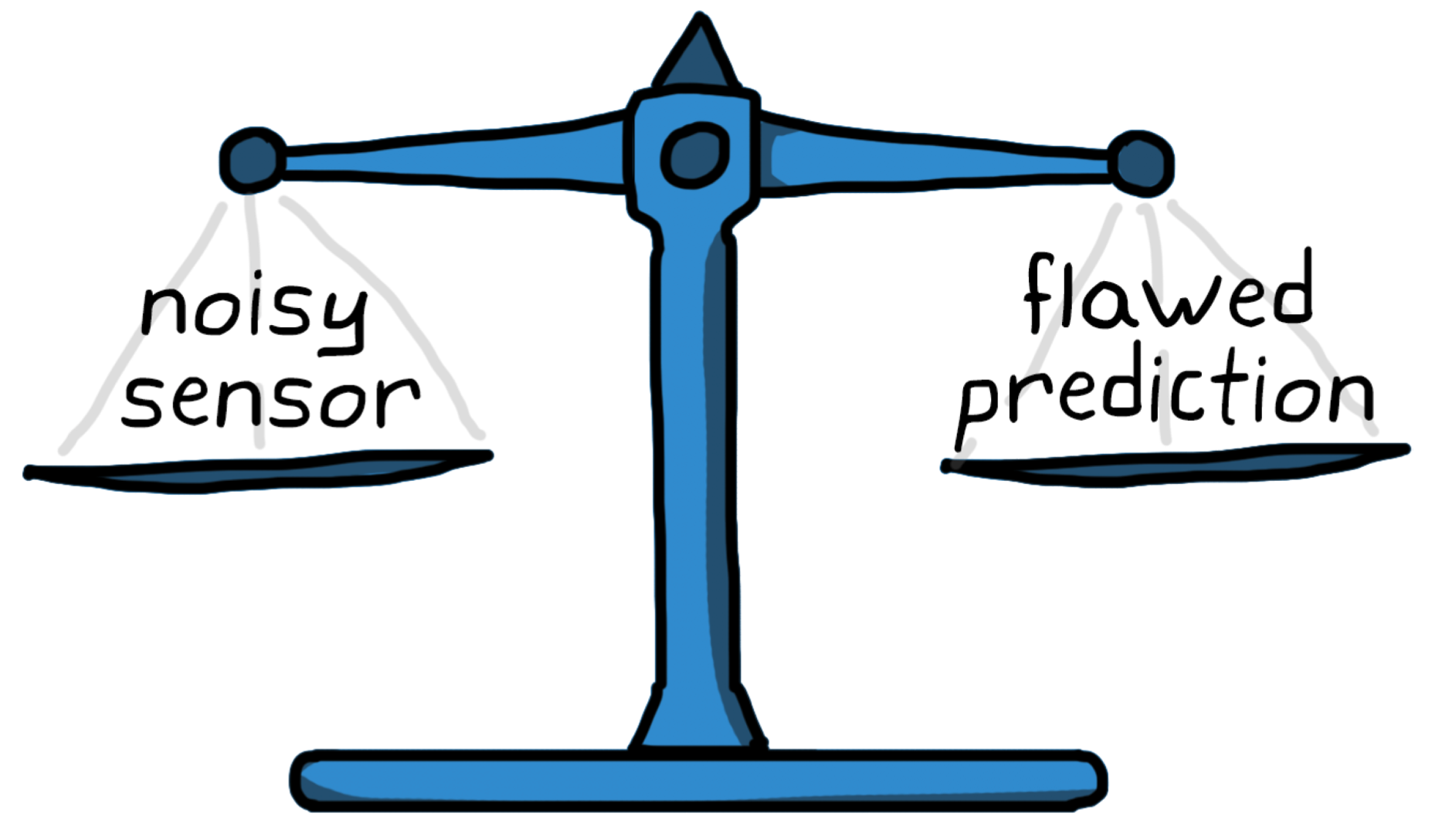
A Kalman filter is an algorithm that we use to estimate the state of a system. It does this by combining a noisy measurement from a sensor with a flawed prediction from a process model. If the measurement noise can be modeled as a Gaussian distribution and the process model can be modeled as linear with a Gaussian error distribution, then a linear Kalman filter will produce an optimal state estimate. The optimal estimation turns out to be the product of the two Gaussian distributions. Therefore, the linear Kalman filter equations can be thought of as a prediction step plus Gaussian multiplication. And I think that’s pretty awesome!
Ok, now on to the full post.
There are many reasons why we want an accurate estimate of the state of a system. One of which is that we need it in feedback control to determine how to change the system. For example, if we are trying to control the temperature of something, we need to have a good estimate of what the current temperature is in order to know if we need to add heat or remove heat from the system.
It’s probably pretty obvious that directly measuring the system with one or more sensors is a way to estimate state, however, what might not be obvious is that we can usually improve our estimate by supplying additional information beyond just what the sensor itself is measuring. One of the methods we have for using some of that additional information is with a Kalman filter.

A Kalman filter is part of a class of estimation filters that use a two-step process, i.e prediction and correction, to produce an optimal state estimate.
If the system can be described with a linear model and the probability distribution of the process noise and measurement noise is Gaussian then a linear Kalman filter will produce the optimal state estimation.
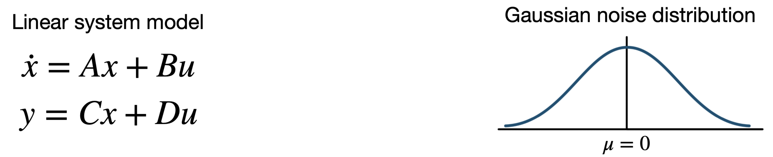
In practice, though, no real system is truly linear and noise might not have a perfect Gaussian probability distribution which means the result of a linear Kalman filter is never absolutely optimal for real systems. However, they still work very well for many real-life problems and the intuition you gain from understanding linear Kalman filters can help you to better understand their nonlinear counterparts like the extended Kalman filter, the sigma-point filter, and the particle filter.
Don’t worry if everything I just described doesn’t mean much to you right now because I’ll touch on some of it a bit more throughout this post. With that being said, let’s walk through a minimal math approach to understanding the linear Kalman filter.
How do people estimate state?
We can start by thinking about how we as humans estimate the state of something. For example, how do we know the velocity of a vehicle, the voltage of an electrical circuit, or the time of day?
The obvious answer is that we measure it directly with a sensor like we do with a speedometer, a voltmeter, or a clock. Similarly, we may derive the state we want by measuring other quantities. This would be the case if we estimate velocity using the difference between two successive position measurements.

But, as humans, we have other knowledge that we use to challenge the validity of our measurements. We have mental models of the world and we use those models to create an expectation of what we’re measuring. And if our expectation differs from the measurement we go through a process of trying to determine which result we trust more. If we trust both results somewhat, but neither fully, then we might blend them together to produce a best guess.
For example, if you look at your watch and it says it’s 4:37 pm and then you wait about a minute, check again, and it says 6:15 pm, you wouldn’t automatically trust that result. We have this general understanding of the passage of time and how the universe should behave and this extra knowledge allows us to make a prediction of how the state of a system should change over some time period. In this case, we would assume our sensor (the watch) was faulty and we’d put more trust in our estimate of the time.

If our model is good, why use measurements at all?
If we have a perfect model and we knew the initial condition of our system, then we would be able to predict how the system state will change over time, perfectly. I mean, why mess around with sensors if we know everything? Well, unfortunately, our ability to predict the outcome of something isn’t perfect, it’s subject to error. This error comes from us having the wrong model of the system and from not knowing and accounting for all of the external inputs that can influence the system state. Therefore, it’s not wise to base the state of the system solely on our flawed prediction. Typically, the longer we predict into the future, the less certain we are in the answer since errors tend to build up over time.
Continuing with the watch example, if you checked your watch and then waited for what you thought was an hour but according to your watch had only been 54 minutes, then you are probably more inclined to believe the measurement and discount your prediction.
This is exactly the thought process behind a Kalman Filter. It combines (in an optimal way) the measurements from a noisy sensor and the prediction from a flawed model to get a more accurate estimate of system state than either one independently could provide.
So, how does the Kalman filter accomplish this?
Let's see some math!
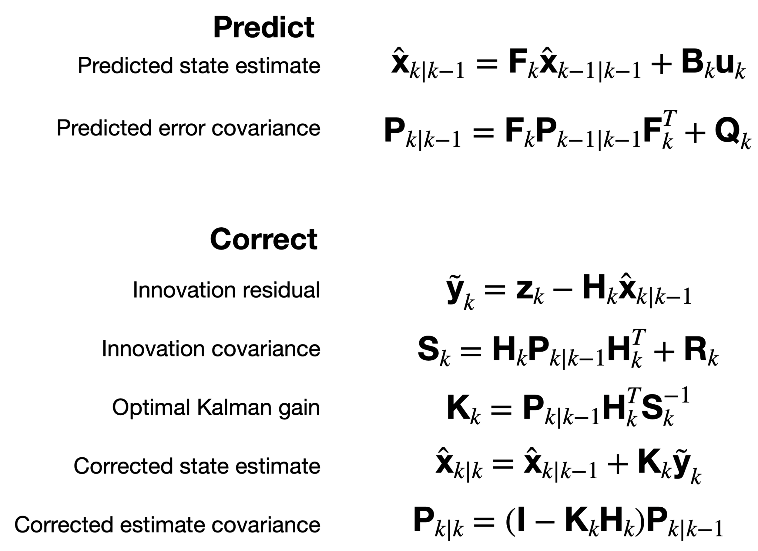
These are the discrete-time equations for a linear Kalman filter. At first glance, they seem complicated and if you’re not familiar with the mathematical notation, then maybe also a bit nonsensical.
They are separated into predict (using the model) and correct (using the measurements), hence the two-step process for estimating state. The predict step is responsible for propagating the state vector into the future using the linear model, and the correct step blends the current prediction with a current measurement to get the corrected estimated state.
Now, rather than try to go through these equations right now, I think they will make a lot more sense if we look at the general idea behind the linear Kalman filter graphically. We’ll come back to these equations afterward.
Less math, let's see some pictures!
Kalman filters and other estimation filters are able to estimate the future state of a system because we give them the ability to predict in the form of a mathematical model. Using this model, the filter propagates the state forward each time step. This is equivalent to us as humans keeping track of the passage of time in our heads.
At some point, the true state is measured with a noisy sensor. We now have two estimates of system state which are likely different; we have a predicted state and a measured state. The question is, which one is correct?
Well, since they both have uncertainty the question really should be, how can we combine the two based on their relative uncertainties?

A Kalman filter determines how much trust, or weight, to apply to both the prediction and the measurement so that the corrected state is placed exactly at the optimal location between the two. This balancing act hinges on a mathematical representation of uncertainty, which we get in the form of covariance.
Variance is a measure of variability
To understand covariance, we need to first look at variance. Informally, variance is a measure of the width of a distribution. It represents how much variability there is in that parameter.
As a simple example, imagine standing at the middle of a field and flipping a coin to determine which direction to step. If it’s heads you walk forward one step and tails you walk backwards one step. After 100 flips, you record how many steps you are from where you started.
Now imagine running this process 10,000 times; always starting at zero and recording where you end up after 100 coin flips. You’re going to create a histogram that looks like this.

We can describe this distribution using three pieces of information.
What is the general shape of the distribution? In our case, this is the classic “bell curve” shape also referred to as a Gaussian distribution or a normal distribution.
Where is the distribution located on the number line? To define this, we can use the average (or mean) value. So, our distribution is located at 0 since it has a mean value of 0 steps.
What is the width of the distribution? In other words, how much variability is there in the distribution. To define this, we can use the standard deviation, σ. In this example it is about 10 steps.
Mathematically, variance is the square of standard deviation and so it’s often written as σ^2. Therefore, our coin flipping process produces a normal distribution with a mean value of 0 steps and a variance of about 100 steps^2.
The reason knowing all of this is important is because we can use these probability distributions to describe the uncertainty in our Kalman filter predictions, the uncertainty in our sensor measurements, and the uncertainty in our mathematical models.
We’ll get to that in just a bit but first if there is more than one parameter we need to keep track of the variances for each of them. For example, we may be interested in the position and velocity of an object and the distribution of each of these variables may be different.

For the sake of this graphical explanation, going forward it may be helpful to represent these unequal variances with an ellipse, where the major and minor axes are set to the variance for that dimension. So, in the below image, this is graphically saying that we have more uncertainty in position than we do in velocity.

Covariance is a generalized variance
Variance doesn’t tell the whole story, however, because something else to consider is that the two states could be correlated. That means that the likelihood of the value of one state depends on the value of another. Therefore, we need to describe covariance.
Let’s go back to our two-state system where we were interested in position and velocity. We could estimate the position and velocity separately and treat the uncertainty in both dimensions according to their respective variances. However, position and velocity are correlated. The faster the object is moving the further the position will travel between measurements. Therefore, know velocity gives us additional information about where to expect position, and knowing position gives us additional information about how fast the object was traveling.
Covariance skews our ellipse in a way that shows the correlation between the two states.

Why draw ellipses when you can create matrices?
We capture this correlation in a covariance matrix. The covariance matrix is a square matrix with the number of rows and columns equal to the number of state variables. So, our position and velocity system would have a 2x2 covariance matrix, P. The diagonal terms are the variance of each state with itself and the off-diagonal terms are the covariances of each state with every other state.

So, if we have two state variables that are not correlated, then the covariance matrix would be diagonal and each term would represent the variance of just that state.
Recap:
A Kalman filter combines a noisy measurement with a flawed prediction to create an optimal state estimate.
We can use covariance as a measure of how much uncertainty there is in the noisy measurement, the flawed model, and the final estimation.
Since covariance is multi-dimensional, it’s mathematically easier to maintain it in matrix form.
A Kalman filter uses three different covariance matrices (measurement, model, final estimation) in order to maintain an estimate of the system state.
Let’s walk through a thought exercise that will explain the different covariance matrices in the filter.
The sensors aren't perfect
The measurement noise covariance matrix, R, captures the expected uncertainty that you have with the sensor measurements. I think the uncertainty in a measurement is pretty easy to understand. There is a true state that we want to know the value of but unfortunately we have to measure it with a noisy sensor.

If we measured the state several times we would see different results from the sensor due to the random noise. This is similar to the coin flipping example from early.

If the noise had zero mean, then the group of measurements would all be centered around the true state. If the noise was Gaussian, then the measurements would follow a normal probability distribution where the width of the distribution, or the amount of noise in the sensor, is the variance.

If all of states that are being measured are uncorrelated, then the measurement covariance matrix would be diagonal and the error ellipse would be aligned with the state variables. This would be the case, for example, with a position sensor who’s x-axis measurement error does not depend on where the system is in the y-axis.

If there is a correlation between the states, then the off-diagonal terms would represent how the value of one measurement affects the uncertainty of another.
The process model isn't perfect
To predict we start at an initial state and then use a mathematical model to propagate that state into the future. There is uncertainty in this whole process. First, the initial state before we even start the prediction process has error. This is captured in the prediction error covariance matrix, P. This means that even with a perfect model, this starting uncertainty will never go away and the final prediction will also have uncertainty associated with it.
Imagine an airplane that is traveling exactly 400 mph and you were asked to predict where it will be in one hour. You know that it will be 400 miles further than the starting position, but if you were uncertain in what that starting position was, then you’d have the same amount of uncertainty in your final answer.
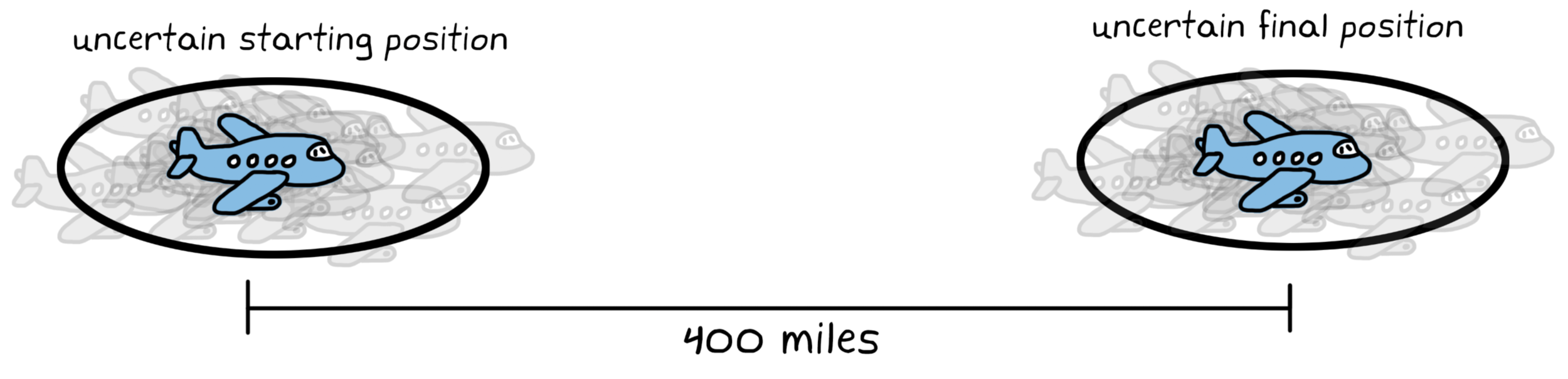
Worse than that, if the model isn’t perfect (which it never is!) the act of predicting into the future causes additional uncertainty. The further into the future we have to predict, the more uncertain it becomes and so the prediction error covariance grows over time.
We specify how the uncertainty grows with the process noise covariance matrix, Q. This matrix captures the uncertainty that comes from model discrepancies and unknown inputs into the system.

Once a Gaussian, always a Gaussian (if linear)
So, we’re keeping track of the uncertainty in the predicted state from the Kalman filter with the prediction error covariance matrix, P.
We’re propagating the predicted state forward with the process model and it’s process noise covariance matrix, Q.
And we’re updating the estimate with our noisy measurements and their measurement noise covariance matrix, R.
It kind of feels like all of this math of combining all of these parts and propagating into the future and everything is going to mess up our nice Gaussian distributions. But luckily - and importantly! - a Gaussian probability distribution maintains its Gaussian shape when subjected to linear operations.
Therefore, if the initial distribution is Gaussian and the process model is linear (or has been linearized prior to running it) then the final prediction uncertainty is still Gaussian in nature. It can be wider or narrower, but it’s just a Gaussian shape. Hence, why Gaussian distributions and linear models are so important for Kalman filters!
So, how do we manage all of this?
We can now frame all of these uncertainties (prediction error covariance, P, process noise covariance, Q, and measurement noise covariance, R) into a single coherent workflow.
At time step K we start with an initial state and its associated error covariance, P, illustrated as an ellipse.

We propagate the state and error covariance into the future (time step k + 1) with a model of the system. The error covariance grows based on the specified process noise covariance, Q.

We continue propagating the prediction each time step. The error covariance will continue to grow, but it will maintain its Gaussian shape.

When a noisy measurement is available, it will have its own uncertainty with a Gaussian distribution that is specified by the measurement noise covariance, R.

At this point, we have a predicted state with an uncertainty described by the prediction error covariance and we have a measured state with an uncertainty described by the measurement noise covariance. Now, we’re back to our question of how to optimally combine these two estimates. Here’s where the magic of the Kalman filter happens. To get the optimal corrected state, all we need to do is … drum roll, please … multiply the two Gaussian distributions together.
The product of two Gaussian is a third Gaussian! The resulting distribution represents the optimal corrected state (the mean of the distribution) and the uncertainty in the result (the covariance of the distribution). Lower covariance means you have more confidence in the estimated state.
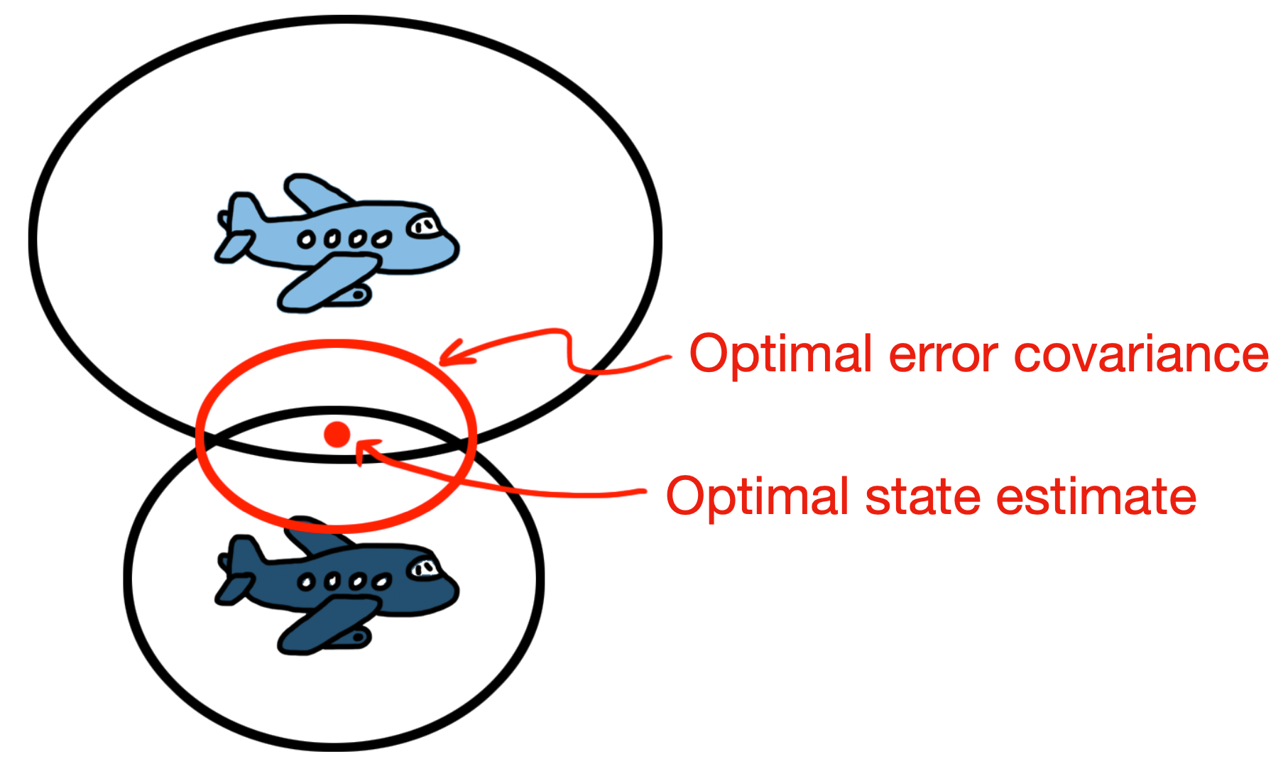
So, now we can think of a Kalman filter as an algorithm that just runs a prediction model and then multiplies two Gaussian distributions: a prediction and its uncertainty distribution with a measurement and its uncertainty distribution.
To really understand the Kalman filter equations, however, we should spend some time expanding on the mathematics of multiplying two Gaussian distributions.
A fast overview of multiplying Gaussians
The equation for a Gaussian distribution is a function of the distribution mean, μ, and its deviation, σ.

Let’s assign μ0 and σ0 for the prediction distribution and μ1 and σ1 for the measurement distribution. Multiplying these two Gaussians together, and sampling the result gives us a new distribution.

The question now is, ‘what does the new mean, μ’, and new variance, σ’^2, look like for the resulting distribution'? If we could solve for them, then we’d know the optimal state estimate and its associated uncertainty.
Unfortunately, solving and simplifying this equation takes more vertical space than I’m willing to devote in this blog post, so we’re just going to jump to the end result since this is really what’s important for what we’re doing. For the proof, check out Theorem 1 and Theorem 2 in this paper by Norbert Freier. It turns out the mean, μ', and variance, σ'^2, of the resulting Gaussian distribution are as follows:
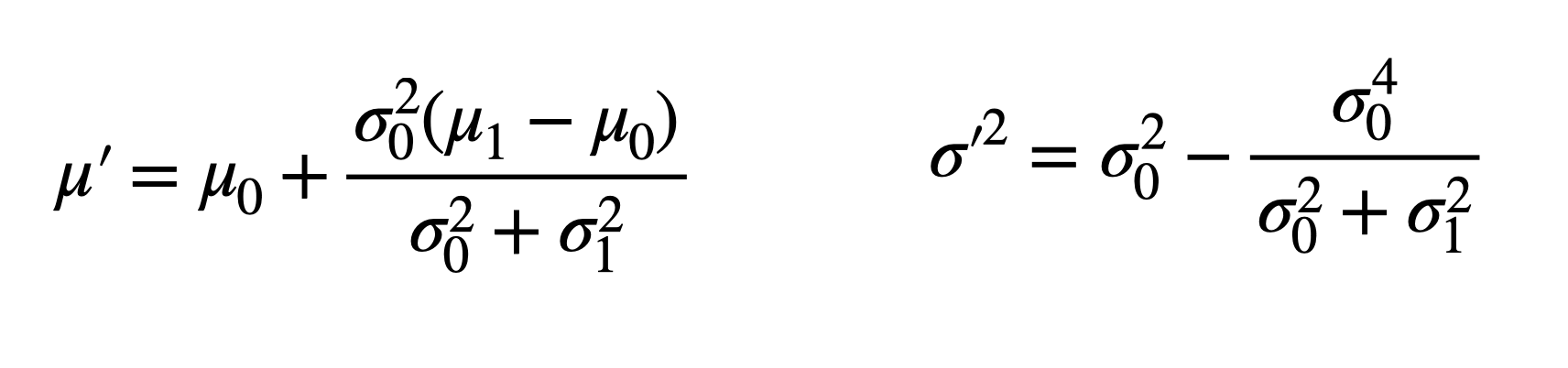
So what is this telling us? If we know the output (mean) of the process model and how much we trust it (variance) and we know the measurement (mean) from the sensor and how much we trust the sensor (variance), then we can combine them with the above equations to produce an optimal estimate.
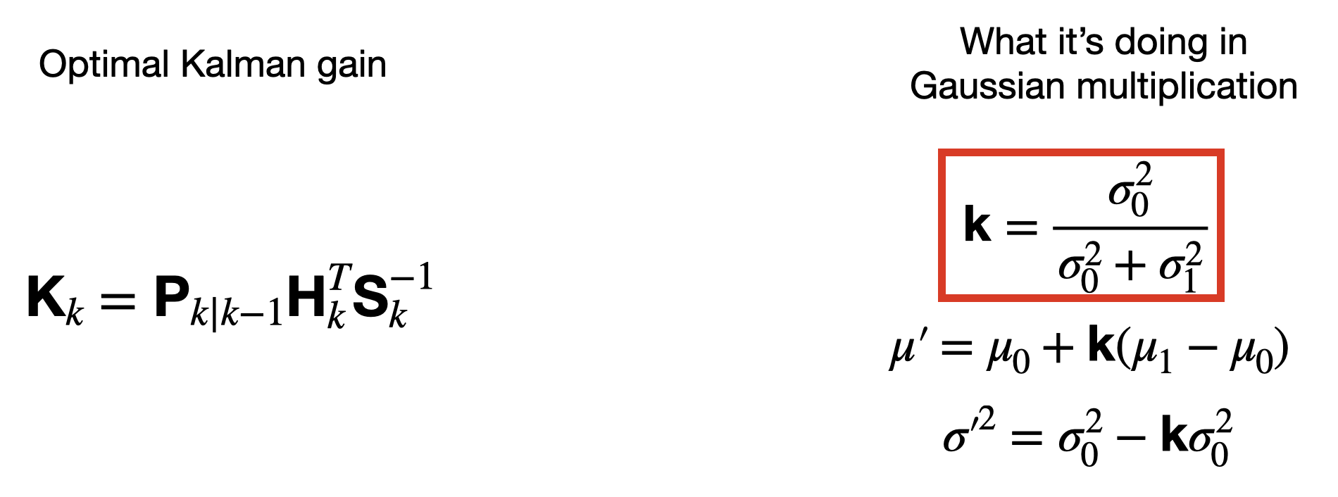
What about the Kalman gain I've heard about?
The equations for the new mean and deviation look complicated, but they have a common multiplier that we can factor out to simplify them. This multiplier, k, is the optimal Kalman gain. The value is a scale between 0 and 1 and it reflects the relative uncertainty in the prediction versus the measurement.

As an interesting aside, let’s assume our sensor measured a value of 5 and it has a variance of 2. And let’s say that our prediction also claims a value of 5 and it also has a variance of 2. It might seem at first that blending these together won’t improve our estimate since they have the same values. However, if you work through the equations you’ll find that the combined estimate will still have the same mean value of 5, but only half of the variance of either individually.

So, in this case, we’ve become more certain of the answer even though the answer has not changed. This make sense because if you have two different methods telling you the same thing, then you should have more confidence that the answer is correct.
ok, I think we're ready for the filter equations again
Now that we know that a Kalman filter simply combines an imperfect prediction it with an imperfect measurement by multiplying two Gaussian functions together, the linear Kalman filter equations that we started with should make more sense. Let’s start with how the filter predicts the estimated future state using the process model.

By accounting for the dynamics of the system and how external control inputs affect the future state, we get a predicted state estimate.
The second part of the predict step is to propagate the error covariance forward. Remember, when we predict, error comes from two different sources: there is the initial uncertainty that we have in the state of the system when we start the prediction and there is the additional uncertainty that is added as we propagate the state forward in time. The longer we propagate, the more uncertain we are in our prediction. This is exactly what this equation is doing.

With the prediction out of the way, we can now focus on using a measurement to correct the predicted state. Each of the equations in the correction step can be understood by recognizing that they accomplish a specific portion of Gaussian multiplication.
The innovation residual is the difference between the output of the sensor, z, and the predicted state, x, rotated into the sensor output frame with H. If the sensor measures the state directly, then H = 1;

The innovation covariance is the sum of the prediction covariance, P, and the measurement covariance, R. Both of these are represented in different frames (state frame versus measurement frame) so P is rotated into the sensor frame using H prior to summation.

The Kalman gain is the ratio of the prediction covariance (in the sensor frame) and the innovation covariance, S, in the sensor frame.
The corrected state estimate is somewhere between the predicted state and the measurement. The predicted state has been "corrected" by the Kalman gain times the innovation residual.

The corrected estimate covariance is less than both the prediction covariance and the measurement covariance as both sets of information is used to improve the uncertainty of the other.

We now have a general understanding of the inner workings of a Kalman filter, however, in order to be able to build one yourself, there are some additional things we need to consider. The goal over the next few sections is not to fully describe everything you need to know in order to set up and run your own Kalman filter (it would require a full book to do it justice), rather, the goal is to introduce you to some of these topics so that at the very least you have them in the back of your mind when you’re tackling your next state estimation problem.
Something to think about when setting up a filter
As we’ve seen, a Kalman filter requires a mathematical model in order to predict the future state. It’s critical that the model is as close to the true nature of the system as possible because any errors, omissions, or inaccuracies degrade the usefulness of the filter.
Think of it this way, if the model is bad then the process noise has to be increased to account for it. This would cause the uncertainty in the prediction to be much greater than the measurement uncertainty since we have less confidence in the model. This would result in the Kalman gain being heavily biased toward the measurement and the prediction would be practically ignored.
Therefore, running a Kalman filter with a very bad model is almost no different than just using the sensor measurements directly.

Since model accuracy is so important, it makes sense that there is an entire field of study surrounding the process of creating a model in the first place.
We touched on measurement noise already, but something we need to think about now is how to build the measurement noise covariance matrix. That is, how do we find the values for our sensors?
A simple solution is to set up a test to have the sensor measure a static quantity and derive the variance from the noisy result. For example, you could place a gyro on an inertially fixed platform and then square the standard deviation from zero rate.
You could do this for every sensor in your system and then the measurement noise matrix could simply be the variance of each sensor along the diagonal.

Another thing to consider is that sensor variance could change while the filter is running based on a real-time estimate of sensor error. For instance, GPS accuracy depends on the number of available satellites and their geometry relative to the receiver. This dilution of precision (DOP) term is generated along with the measured position and can be used to adjust the variance for that single measurement.

The process noise covariance matrix needs to account for unknown inputs and modeling discrepancies but this is a bit trickier to measure or estimate. It can be hard to quantify how far off your model is from the truth if you’re not able to know how the real system will behave in every operational scenario.
One way to approach this is to run the physical system in the real operational environment. Then you could compare its behavior to your model operating under the same environment conditions. The variance could be calculated once again by looking at the standard deviation of the error.

Often, when you hear the phrase "tuning a Kalman filter" it means you’re tweaking the process noise and measurement noise matrices and trying to find something that produces acceptable results. And, typically, the matrix you spend the most time on depends on if it’s the model or the sensors that is harder to understand.
Another aspect of the Kalman filter that we have control over is how to initialize it. We need an initial state and covariance so that the prediction step has somewhere to begin. If we’re using a linear Kalman filter we can pretty much choose any state we want and it’ll converge eventually - it’ll just take more time if it’s initialized too far from the truth.

However, that’s not the case for an Extended Kalman Filter (EKF). An EKF propagates state and covariance using a nonlinear model. It works by linearizing the model around its current estimate and then using that linear model to propagate the state into the future. If the filter is not initialized close enough to the true state, the linearization process could be so far off that it causes the filter to never actually converge. Therefore, it’s important to find a way to get an accurate initial state.

There are a few ways to initialize an estimation filter with an acceptable initial state. One is to simply initialize the filter with a predetermined, hard-coded state and just ensure that the system is in that state when the filter starts running. For example, you could use a jig or other markings in the environment that will ensure the system is placed in the expected state.

Another way is to set the initial state using the raw measurements from the sensors. The sensors will have noise and other errors, but the hope is that they still provide a measurement close enough to the truth that the filter can converge.

This brings us to the concept of convergence. If you don’t have a good initial estimate of the system state when you start your filter, then it makes sense that you can’t trust the results right away. You have to give it some time to read the sensors and run the correction step - possibly many correction steps - before the estimated state and covariance are close to the truth.
For example, the plots below show a hypothetical estimated velocity for an object that is not accelerating. You’d expect the output from the Kalman filter to show a fixed velocity, however, the accelerometer has a slight positive bias that isn’t accounted for. The Kalman filter is set up to estimate bias but it’s been initialized to 0 m/s2. When the filter is running, a second sensor measures the velocity of the object directly and is used to correct the estimated state. Each correction step both the velocity and the accelerometer bias are updated. The bias error is lowered over time and eventually matches the true sensor bias. At this point, the filter has converged and the output can be trusted.

Continue reading: Coming soon (maybe but probably not too soon)
Previous post: #1: What is control engineering?
This post was influenced by the fantastic article, How a Kalman filter works in pictures by Tim Babb. I recommend you check it out!